大学キャンパスで感染拡大を抑制するための最適化

導入: パンデミック時代に、組合せ最適化ができること

2019年末より世界で始まったCOVID-19感染拡大は、これまでの人々の生活を一変させました。このパンデミックにより、大学生はキャンパスへの入場が一時的に制限されました。Sud & Li, 2021では、大学キャンパスの学生グループを物理的な感染拡大防止のコホートにマッピングするための、量子アニーリングを用いた最大カット問題の再帰的解法を考案しました。今回はこのアルゴリズム実装に、JijModelingとJijZeptSolverを用いてみましょう。またそのコホートから実際に感染症モデルを解き、感染がどの程度広がるかを見てみましょう。

アルゴリズム

学生をいくつかのグループに分割し、キャンパスに登校する日や使用する教室を分けることで、感染の拡大を防止します。そのために、学生の繋がりをグラフとして考えましょう。そのグラフの最大カット問題を解き、グラフを2つに分けます。

最大カット問題を解くことを繰り返し、欲しい数のコホートに到達したら、その時点で繰り返しを終了します。

G = 入力ネットワークグラフ
N = 希望するコホート数 // ここでは2のべき乗とします
currCohorts = [G]
while currCohortsの長さがNより小さい間:
    newCohorts = []
    for c in currCohorts:
        c1, c2 = performMaxcut(c) // 最大カット問題で、グラフを2つに分割
        newCohorts.append(c1)
        newCohorts.append(c2)
    currCohorts = newCohorts

後述するperformMaxcut関数は、最大カット問題を解き、グラフを2つに分割する関数です。論文ではD-Waveの量子アニーラを用いていますが、今回はこの部分にJijModeling, そしてJijZeptSolverを用いましょう。

最大カット問題の数理モデル

グラフ\(c = (V, E)\)を2つに分割する際に、最大カット問題を解いています。ここではその定式化について考えてみましょう。\(c\)に属する頂点をプラス・マイナスの2つの集合に分けます。このとき、切断するエッジの重みの総和が最大となるような分け方を求める問題です。

カットする辺の重みが最大となるようにする

頂点\(i\)がプラス集合に属するとき\(s_i = 1\)、マイナス集合に属するとき\(s_i = -1\)となるようなスピン変数を与えます。カットする辺の重みが最大となるように考えます。頂点\(i\)と頂点\(j\)を結ぶ辺の持つ重みを\(w_{ij}\)のように書きます。プラス集合に属する頂点とマイナス集合に属する頂点の間のみについて考えるため、その総和は

\[ \mathrm{obj} = - \sum_{(i, j) \in E} \frac{w_{ij}}{2} (1-s_i s_j) \tag{1} \]

のように書かれます。\(s_i = s_j \)のとき、\(1-s_i s_j = 0\)となるため、\(s_i \neq s_j\)の辺の重みだけが加算されていくことを表現したものです。今回の問題では\(w_{ij} = 1\)のようにします。すなわち、純粋に学生を2つのグループに分けることを考えます。

バイナリ変数との対応

JijModelingはバイナリ変数にのみ対応しているため、スピン変数との対応を考える必要があります。頂点\(i\)がプラス集合に属するとき\(x_i = 1\)、マイナス集合に属するとき\(x_i = -1\)となるようなバイナリ変数を考えましょう。すると、\(s_i \)と\(x_i\)の対応は

\[ x_i = \frac{1+s_i}{2} \ \Longrightarrow \ s_i = 2 x_i - 1 \tag{2} \]

のようになります。

実装しましょう

ここからは、実際にJijModelingとJijZeptSolverを用いて、この問題を解くスクリプトを実装しましょう。

変数の定義

以下のようにして、最適化に用いる変数を定義します。

import jijmodeling as jm

problem = jm.Problem('Max cut')

V = problem.Natural('V')
E = problem.Graph('E')
w = problem.Float('w', shape=(V, V))
x = problem.BinaryVar('x', shape=(V,))

Vはグラフ頂点数、Eは辺集合、wはグラフの重み、そしてxはバイナリ変数を表します。

最大カット問題の実装

次に、最大カット問題の目的関数式(1)を実装しましょう。

# set objective function: maximize the cut-edge weights
problem += - jm.sum(E, lambda e: 0.5 * w[e[0], e[1]] * (1 - (2 * x[e[0]] - 1) * (2 * x[e[1]] - 1)))

途中、2つのスピン変数を定義し、それを用いて式(1)の実装を行なっています。
Jupyter Notebook上で、実装した数理モデルを確認しましょう。

problem

\[\begin{split}\begin{array}{rl} \text{Problem}\colon &\text{Max cut}\\\displaystyle \min &\displaystyle -\sum _{e\in E}{0.5\cdot {w}_{{e}_{0},{e}_{1}}\cdot \left(1-\left(2\cdot {x}_{{e}_{0}}-1\right)\cdot \left(2\cdot {x}_{{e}_{1}}-1\right)\right)}\\&\\\text{where}&\\&\text{Decision Variables:}\\&\qquad \begin{alignedat}{2}x&\in \mathop{\mathrm{Array}}\left[V;\left\{0, 1\right\}\right]&\quad &1\text{-dim binary variable}\\\end{alignedat}\\&\\&\text{Placeholders:}\\&\qquad \begin{alignedat}{2}E&\in \mathop{\mathrm{Array}}\left[(-);\mathbb{N}\times \mathbb{N}\right]&\quad &1\text{-dimensional array of placeholders with elements in }\mathbb{N}\times \mathbb{N}\\V&\in \mathbb{N}&\quad &\text{A scalar placeholder in }\mathbb{N}\\w&\in \mathop{\mathrm{Array}}\left[V\times V;\mathbb{R}\right]&\quad &2\text{-dimensional array of placeholders with elements in }\mathbb{R}\\\end{alignedat}\end{array} \end{split}\]

グラフ生成

大学キャンパスなど、複数の人間が形成するネットワークを模倣したグラフを作成しましょう。 ここではWatts & Strogatz, 1998で提案されたsmall-worldグラフを採用します。

import networkx as nx

# set a small-world graph
inst_V = 1000
k = 20
p = 0.1
inst_G = nx.watts_strogatz_graph(inst_V, k, p)
# set weights on the edges
for edge in inst_G.edges:
    inst_G[edge[0]][edge[1]]['weight'] = 1.0

JijZeptSolverで解く

jijzept_solverを用いて、最大カット問題を解きましょう。 最大カット問題を反復するための関数を作成します。

import jijzept_solver
import numpy as np

# A function to prepare a graph instance for MaxCut
def make_instance(input_c):
    # get the number of nodes
    inst_V = len(input_c.nodes)
    # relavel name of nodes
    mapping_dict = {a: b for a, b in zip(input_c.nodes, range(inst_V))}
    c = nx.relabel_nodes(input_c, mapping_dict)
    # get edges and weights
    inst_E = [[edge[0], edge[1]] for edge in c.edges]
    inst_w = np.zeros([inst_V, inst_V])
    for k, v in nx.get_edge_attributes(c, 'weight').items():
        inst_w[k[0], k[1]] = v
    return {'V': inst_V, 'E': inst_E, 'w': inst_w}

# A function to make two graphs from JijZept results
def make_graph(solution, c):
    df = solution.decision_variables_df
    x_indices = np.ravel(df[df["value"]==1]["subscripts"].to_list())
    # extract a subgraph (x=1) from original graph
    c1 = c.copy()
    c1 = c1.subgraph(x_indices)
    # remove a subgraph from the original graph
    c2 = c.copy()
    c2.remove_nodes_from(x_indices)
    return c1, c2

# execute MaxCut
def performMaxcut(c):
    instance_data = make_instance(c)
    # compute the Max-Cut using JijZeptSolver
    instance = problem.eval(instance_data)
    solution = jijzept_solver.solve(instance, solve_limit_sec=1.0)
    return make_graph(solution, c)

上述の関数を用いて、繰り返し最大カット問題を解きましょう。

# set the number of cohorts
N = 4
currCohorts = [inst_G, ]
# iteration
while len(currCohorts) < N:
    newCohorts = []
    for c in currCohorts:
        c1, c2 = performMaxcut(c)
        newCohorts.extend([c1, c2])
    currCohorts = newCohorts

この計算により、N個に分割されたグラフを得ることができます。

感染症モデルへの入力

感染症のよく知られたモデルの一つに、Kermack & McKendrick (1927)で導入されたSIRモデルがあります。 このモデルは、以下の3つの微分方程式からなるモデルです。

\[ \frac{dS}{dt} = -\beta S I \tag{3} \]

\[ \frac{dI}{dt} = \beta S I - \gamma I \tag{4} \]

\[ \frac{dR}{dt} = \gamma I \tag{5} \]

ここで\(S\)はsusceptible(未感染者: これから感染する可能性を持つ)、\(I\)はinfectious(感染者: 他人に移す可能性を持つ)、\(R\)はrecovered(既感染者: 感染から回復し免疫を持つ)を表します。またパラメータである\(\beta, \gamma\)はそれぞれ感染症の感染率と回復率を表す定数です。COVID-19においては平均の回復期間が\(Tr\) = 10daysと判明していることから、大雑把に\(\gamma = 1/ Tr\)と与えます。また感染者が感染している間に感染を移す平均人数を\(\alpha\)のように書くと、これは

\[ \alpha = \mathrm{avg\_deg}(G) \times \frac{\beta}{\gamma} \tag{6} \]

のように書くことができます。ここで\(\mathrm{avg\_deg}(G)\)は、学生の繋がりを表すグラフ\(G\)の平均の次数を表します。COVID-19では\(1.5 \leq \alpha \leq 6.7\)と判明しているため、(6)式からモデル計算を行うグラフ\(G\)を与えれば、\(\beta\)を見積もることが可能です。これらを学生の繋がりを表すグラフに合わせて解くことで、そのキャンパスで感染症がどのように広がるかをモデル化することができます。ここでは、先程のアルゴリズムにより分割された学生のコホートをこのモデルに入力し、感染者数の推移などを見ていきましょう。そのために、グラフのトポロジーも考慮してSIRモデルを解く機能を持つNDlibライブラリを利用します。

import ndlib.models.ModelConfig as mc
import ndlib.models.epidemics as ep

# a function for solving SIR model
def solveSIR(g):
    # compute average degree of a graph
    list_degree = [g.degree[n] for n in g.nodes()]
    avg_deg = sum(list_degree) / len(list_degree)
    # set parameters for SIR model
    gamma = 1.0 / 10
    alpha = 3.0
    beta = alpha * gamma / avg_deg
    # set SIR model
    model = ep.SIRModel(g)
    # input parameters
    cfg = mc.Configuration()
    cfg.add_model_parameter('beta', beta)
    cfg.add_model_parameter('gamma', gamma)
    cfg.add_model_parameter('percentage_infected', 0.05)
    model.set_initial_status(cfg)
    # compute SIR model
    iterations = model.iteration_bunch(100)
    trends = model.build_trends(iterations)
    return model, trends

比較のために、MaxCutを用いて分割した場合と、ランダムにグラフを分割した場合の計算結果を可視化したものを以下に示します。

from ndlib.viz.mpl.DiffusionTrend import DiffusionTrend
from ndlib.viz.mpl.TrendComparison import DiffusionTrendComparison
import random
import matplotlib.pyplot as plt

# Enable inline plotting for Jupyter
%matplotlib inline

# solve the SIR model
model1, trends1 = solveSIR(currCohorts[0])

cohort_idx = 0
list_random_partition_nodes = []
for i in inst_G.nodes:
    if random.randint(0, N-1) == cohort_idx:
        list_random_partition_nodes.append(i)
G_temp = inst_G.copy()
random_g = G_temp.subgraph(list_random_partition_nodes)
# solve the SIR model
model2, trends2 = solveSIR(random_g)

viz = DiffusionTrendComparison([model1, model2], [trends1, trends2], "Infected")
viz.plot()
plt.show()

no display found. Using non-interactive Agg backend
no display found. Using non-interactive Agg backend

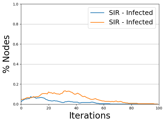
青線はMaxCut、オレンジ線はランダム分割の場合の感染者数の推移を表しています。 MaxCutを用いた場合の方が、感染者数が少ないことがわかります。 実際に大学キャンパスにおける人同士の接触をグラフ化し、それをこの手法にしたがって分割します。 分割により作成されたグループごとにキャンパスへの登校日を変えれば、感染拡大を防ぐことができるとわかります。

参考文献

• Sud & Li, 2021, "A Quantum Annealing Approach to Reduce Covid-19 Spread on College Campuses"

• Watts & Strogatz, 1998, "Collective dynamics of 'small-world' networks"

• Kermack & McKendrick, 1927, "A contribution to the mathematical theory of epidemics"

• Rossetti et al., 2017, "NDLIB: a python library to model and analyze diffusion processes over complex networks"