整数長ジョブシーケンス問題

ここではJijZeptSolverとJijModelingを用いて、長さが整数のジョブシーケンス問題を解いてみましょう。 この問題は、Lucas, 2014, "Ising formulations of many NP problems"の6.3. Job Sequencing with Integer Lengthsでも触れられています。

整数長ジョブシーケンス問題とは

タスク1は1時間の実行時間、タスク2は3時間の実行時間、のように、整数長のタスクがいくつかあるような場合を考えましょう。 「これらのタスクを複数コンピュータに分散させる場合、偏りを生じさせることなく、これらのコンピュータの実行時間を最適に分散させるにはどうすれば良いか？」を求める問題です。

例

次のような問題を考えてみましょう。

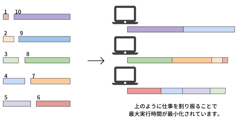
10個のタスクを、3台のコンピュータに分散させることを考えましょう。 10個のタスクの長さはそれぞれ、1, 2, ..., 10であるとします。 私たちの目的は、3つのコンピュータの最大実行時間を、最小化するような解を求めることです。 この場合、最適解は\(\{1, 2, 7, 8\}, \{3, 4, 5, 6\}, \{9, 10\}\)などがあり、この場合のコンピュータ実行時間の最大値は19となります。

一般化

次に、\(N\)個のタスク(\(\{0, 1, \dots, N-1\}\))について考えることにしましょう。 これらのタスクの実行時間は\(L= \{L_0, L_1, \dots, L_{N-1}\}\)とします。 \(M\)個のコンピュータが与えられたとき、\(j\)番目のコンピュータに割り当てられたタスクの集合を\(V_j\)としたとき、\(j\)番目のコンピュータに割り当てられたタスクの総実行時間は\(A_j = \sum_{i \in V_j} L_i\)のようになります。 そして\(i\)番目のタスクを\(j\)番目のコンピュータに割り当てるとき1、そうでないとき0となるバイナリ変数を\(x_{i, j}\)のように書くことにしましょう。

制約: 各タスクはいずれか1つのコンピュータに割り当てられなければならない

例えば、5番目のタスクを、1番目と2番目のコンピュータに同時に割り当てることはできません。 これを数式で表現すると、以下のようになります。

\[ \sum_{j=0}^{M-1} x_{i, j} = 1 \quad (\forall i \in \{0, 1, ..., N-1\}) \tag{1} \]

目的関数: 0番目のコンピュータと他のコンピュータとの層実行時間の差を最小化する

0番目のコンピュータの総実行時間を基準として扱い、それと他のコンピュータとの差を最小化することを考えましょう。 これにより、実行時間のばらつきが小さくなり、タスクが均等に分散されます。

\[ \min \quad \sum_{j=1}^{M-1} (A_0 - A_j)^2 \tag{2} \]

JijModelingを用いたモデル化

次に、JijModelingを用いた実装を説明します。 まずは上述の数理モデルで用いる変数を定義しましょう。

import jijmodeling as jm

problem = jm.Problem('Integer Jobs')

# defin variables
L = problem.Float('L', ndim=1)
N = problem.DependentVar("N", L.len_at(0))
M = problem.Natural('M')
x = problem.BinaryVar('x', shape=(N, M))

Lは各タスクの実行時間を表す1次元配列です。 Nはタスク数を表します。 Mはコンピュータの数を表します。 そして、\(x\)は2次元のバイナリ変数列を表します。

制約

式(1)の制約を実装しましょう。

# set constraint: job must be executed using a certain node
problem += problem.Constraint('onehot', lambda i: jm.sum(M, lambda j: x[i, j]) == 1, domain=N)

目的関数

次に、式(2)の目的関数を実装します。

# set objective function: minimize difference between node 0 and others
A_0 = jm.sum(N, lambda i: L[i]*x[i, 0])
problem += jm.sum(
    jm.filter(lambda j: j != 0, M),
    lambda j: (A_0 - jm.sum(N, lambda i: L[i]*x[i, j])) ** 2,
)

jm.filter(lambda j: j != 0, M) は\(j \neq 0\)以外の\(j\)を取ることを意味します。

実装した数理モデルを、Jupyter Notebook上で表示してみましょう。

problem

\[\begin{split}\begin{array}{rl} \text{Problem}\colon &\text{Integer Jobs}\\\displaystyle \min &\displaystyle \sum _{\substack{j=0\\j\neq 0}}^{M-1}{{\left(\sum _{i=0}^{N-1}{{L}_{i}\cdot {x}_{i,0}}-\left(\sum _{i=0}^{N-1}{{L}_{i}\cdot {x}_{i,j}}\right)\right)}^{2}}\\&\\\text{s.t.}&\\&\begin{aligned} \text{onehot}&\quad \displaystyle \sum _{j=0}^{M-1}{{x}_{i,j}}=1\quad \forall i\;\text{s.t.}\;i\in \left\{0,\ldots ,N-1\right\}\end{aligned} \\&\\\text{where}&\\&\text{Decision Variables:}\\&\qquad \begin{alignedat}{2}x&\in \mathop{\mathrm{Array}}\left[N\times M;\left\{0, 1\right\}\right]&\quad &2\text{-dim binary variable}\\\end{alignedat}\\&\\&\text{Placeholders:}\\&\qquad \begin{alignedat}{2}L&\in \mathop{\mathrm{Array}}\left[(-);\mathbb{R}\right]&\quad &1\text{-dimensional array of placeholders with elements in }\mathbb{R}\\M&\in \mathbb{N}&\quad &\text{A scalar placeholder in }\mathbb{N}\\\end{alignedat}\\&\\&\text{Dependent Variables:}\\&\qquad \begin{alignedat}{2}N&=\mathop{\mathtt{len\_{}at}}\left(L,0\right)&\quad &\in \mathbb{N}\\\end{alignedat}\end{array} \end{split}\]

インスタンスの準備

各ジョブの実行時間と、コンピュータ数を設定しましょう。 ここでは、先ほど述べた10個のタスクと3台のコンピュータの場合を用います。

# set a list of jobs
inst_L = [1, 2, 3, 4, 5, 6, 7, 8, 9, 10]
# set the number of Nodes
inst_M = 3
instance_data = {'L': inst_L, 'M': inst_M}

JijZeptSolverで解く

jijzept_solverを用いて、この問題を解いてみましょう。

import jijzept_solver

instance = problem.eval(instance_data)
solution = jijzept_solver.solve(instance, solve_limit_sec=1.0)

解の可視化

最後に、得られた解を可視化してみましょう。

import matplotlib.pyplot as plt
import numpy as np

df = solution.decision_variables_df
x_indices = df[df["value"]==1]["subscripts"].to_list()
# get the instance information
L = instance_data["L"]
M = instance_data["M"]
# initialize execution time
exec_time = np.zeros(M, dtype=np.int64)
# compute summation of execution time each nodes
for i, j in x_indices:
    plt.barh(j, L[i], left=exec_time[j],ec="k", linewidth=1,alpha=0.8)
    plt.text(exec_time[j] + L[i] / 2.0 - 0.25 ,j-0.05, str(i+1),fontsize=12)
    exec_time[j] += L[i]
plt.yticks(range(M))
plt.ylabel('Computer numbers')
plt.xlabel('Execution time')
plt.show()

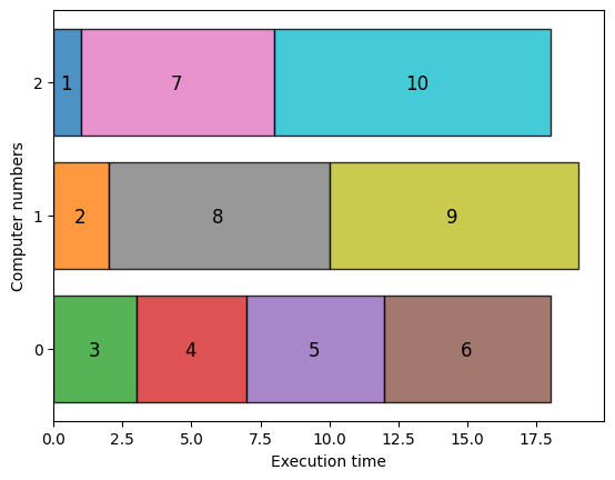
可視化されたグラフから、実行時間が3台のコンピュータに分散されていることがわかります。 この場合の実行時間の最大値は19であることから、最適解が得られていることもわかります。