グラフ同型問題#
ここではJijZeptSolverとJijModelingを用いて、グラフ同型問題を解く方法を説明します。 この問題は、Lucas, 2014, "Ising formulations of many NP problems" 9. Graph Isomorphisms でも触れられています。
グラフ同型問題とは#
グラフ同型問題は、2つのグラフ\(G_1, G_2\)が同じ構造を持っているかどうかを判定する問題です。 すなわち、\(N\)個の頂点と辺が同じ数かつ、それらの頂点と辺が同じ配置かどうかを判定します。 詳しく見ていきましょう。 \(1, \dots, N\)のラベルが付けられた頂点を持つグラフ\(G=(V, E)\)に対し、\(N \times N\)の隣接行列\(A\)を次のように定めます。
この辺集合\(E\)について、制約を考えていきましょう。
数理モデル#
最初に、グラフ\(G_2\)内の頂点\(v\)がグラフ\(G_1\)の頂点\(i\)にマッピングされるとき1、そうでないとき0となるようなバイナリ変数\(x_{v, i}\)を導入しておきましょう。
制約 1: グラフ間のマッピングは全単射 (一対一対応) でなければならない#
2つのグラフ間の全単射マッピングとは、2つのグラフの頂点間が一対一対応でなければならないという意味です。 すなわち、片方のグラフの各頂点は、もう片方のグラフにおける頂点とペアになる必要があります。
制約 2: 存在しないマッピング#
\(G_1\)には存在しない辺が\(G_2\)に存在する、\(G_1\)に存在する辺が\(G_2\)に存在しない辺があるようなことは、避けなければなりません。
JijModelingによる定式化#
次に、JijModelingを用いた実装を示します。 最初に、上述の数理モデルで必要な変数を定義します。
import jijmodeling as jm

# set problem
problem = jm.Problem('Graph Isomorphisms')

# define variables
V = problem.Natural('V')  # number of vertices
E1 = problem.Graph('E1', dtype=V)  # set of edges
E2 = problem.Graph('E2', dtype=V)  # set of edges
E1_bar = problem.Graph('E1_bar', dtype=V)
E2_bar = problem.Graph('E2_bar', dtype=V)

x = problem.BinaryVar('x',shape=(V, V))
E1とE2は、グラフ\(G_1\)と\(G_2\)の辺の集合を表すプレースホルダ変数です。
E1_barとE2_barは、それぞれのグラフの補グラフの辺の集合を表すプレースホルダ変数です。
インスタンスを構築する時に、これらのプレースホルダ変数の値として、E1とE2の補グラフの辺の集合が実際に渡されるよう注意しなければなりません。
制約#
次に、制約の式を実装しましょう。
# set constraint
problem += problem.Constraint('const1-1', lambda v: jm.sum(V, lambda j: x[v, j])==1, domain=V)
problem += problem.Constraint('const1-2', lambda i: jm.sum(V, lambda v: x[v, i])==1, domain=V)

const2_1 = jm.sum(jm.product(E1_bar, E2), lambda f1, e2: x[e2[0],f1[0]]*x[e2[1],f1[1]])
const2_2 = jm.sum(jm.product(E1, E2_bar), lambda e1, f2: x[f2[0],e1[0]]*x[f2[1],e1[1]])
problem += problem.Constraint('const2', const2_1 + const2_2==0)
Jupyter Notebook上で、実装した数理モデルを表示してみましょう。
problem
インスタンスの準備#
Networkxを用いて、グラフを準備しましょう。
import networkx as nx
import numpy as np
import matplotlib.pyplot as plt

# First graph
graph1 = [[0, 1, 0, 1],
          [1, 0, 1, 0],
          [0, 1, 0, 1],
          [1, 0, 1, 0]]

# Second graph
graph2 = [[0, 0, 1, 1],
          [0, 0, 1, 1],
          [1, 1, 0, 0],
          [1, 1, 0, 0]]

# Create networkx graphs from adjacency matrices
G1 = nx.from_numpy_array(np.array(graph1))
G2 = nx.from_numpy_array(np.array(graph2))

num_V = G1.number_of_nodes()

edges1 = G1.edges()
inst_E1 = [list(edge) for edge in edges1]

edges2 = G2.edges()
inst_E2 = [list(edge) for edge in edges2]

non_edges1 = list(nx.non_edges(G1))
inst_E1_bar = [list(non_edge) for non_edge in non_edges1]

non_edges2 = list(nx.non_edges(G2))
inst_E2_bar = [list(non_edge) for non_edge in non_edges2]

instance_data = {'V': num_V, 'E1': inst_E1, 'E2': inst_E2, 'E1_bar': inst_E1_bar, 'E2_bar': inst_E2_bar}
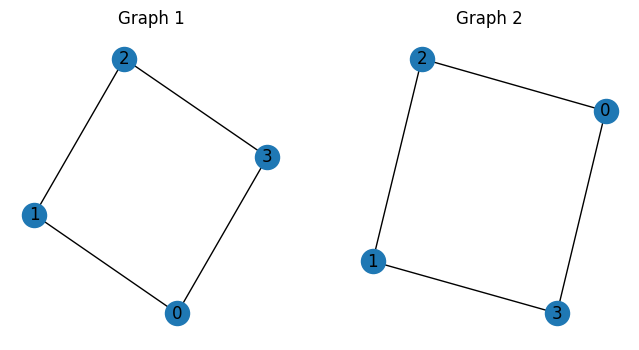
用意したグラフを可視化すると、以下のようになります。
# Create figure and subplots
fig, axs = plt.subplots(1, 2, figsize=(8, 4))

# Draw graphs
nx.draw(G1, ax=axs[0], with_labels=True)
axs[0].set_title("Graph 1")
nx.draw(G2, ax=axs[1], with_labels=True)
axs[1].set_title("Graph 2")

# Show the plot
plt.show()
JijZeptSolverで解く#
jijzept_solverを用いて、問題を解きましょう。
import jijzept_solver

instance = problem.eval(instance_data)
solution = jijzept_solver.solve(instance, solve_limit_sec=1.0)
解のチェック#
最後に、得られた解をチェックしてみましょう。
df = solution.decision_variables_df
x_indices = df[df["value"]==1]["subscripts"].to_list()
vertices, orders = zip(*x_indices)
print(f'vertex: {vertices}')
print(f'orders: {orders}')
vertex: (0, 1, 2, 3)
orders: (0, 2, 3, 1)
期待通り、JijZeptSolverにより2つのグラフが同型であることが示されました。