有向フィードバック頂点集合問題

ここではJijZeptSolverとJijModelingを用いて、有向フィードバック頂点集合問題を解く方法を説明します。 この問題は、Lucas, 2014, "Ising formulations of many NP problems" 8.3. Directed Feedback Vertes set でも触れられています。

有向フィードバック頂点集合問題とは

有向フィードバック頂点集合とは、有向グラフ \(G = (V, E)\) において頂点を取り除いたときに、そのグラフが非巡回グラフ (つまりどのような巡回も含まないグラフ) になるような頂点集合を意味します。 言い換えれば、有向グラフにおけるフィードバック頂点集合とは、部分グラフ \((V-F, \partial (V-F))\) が非巡回グラフとなるような部分頂点集合 \(F \subset V\) となるような集合を見つける問題です。 ここで\(F\)をフィードバック集合としました。 このフィードバック集合が最小サイズとなるように、最適化問題を解いてみましょう。

例題

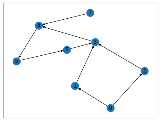
次のような有向グラフ \(G = (V, E)\) と、そのグラフにおけるフィードバック頂点集合を考えてみましょう。 このグラフにおけるフィードバック頂点集合は \(F = \{ 3 \}\) ただ一つです。 この頂点\(3\)をグラフから取り除くと、残された部分グラフ \(\{0, 1, 2, 4, 5, 6, 7\}\)は非巡回グラフとなることがわかります。

有向非巡回グラフにおいて、自分自身の頂点を指す辺を持たない頂点の存在

有向非巡回グラフには、どの辺の端点にならない頂点が存在します。 これは、辺の向きに沿ってグラフの辺をたどっても、出発点と同じ頂点に行き着くことができないことを意味します。

有向グラフの条件

有向グラフの条件は、高さ \(h: V \to N\) から考えることができます。 これは全ての辺に対して \((uv) \in E\), \(h(u) < h(v)\)となるように、グラフ各点に非負の整数を割り当てるものです。 言い換えれば、任意の有向辺の開始点は、終点より低い高さとなります。

数理モデルの構築

最初に、頂点\(v\)がフィードバック集合に含まれるとき0、そうでないとき1となるようなバイナリ変数\(y_v\)を導入しましょう。 さらに、頂点\(v\)が高さ\(i\)のとき1、そうでないとき0となるようなバイナリ変数\(x_{v, i}\)も用いることにします。

制約 1: フィードバック集合でない頂点は、高さが定まってなければならない

これを数式で表すと、以下のようになります。

\[ \quad y_v - \sum_ix_{v,i} = 0 \quad (\forall v) \tag{1} \]

制約 2: 辺は高さが低い頂点から高い頂点へと結ばれてなければならない

これを数式で表現すると、次のようになります。

\[ \quad \sum_{(uv) \in E}\sum_{i \geq j}x_{u,i}x_{v,j} = 0 \tag{2} \]

目的関数: フィードバック集合のサイズを最小化する

目的関数は、次のようになります。

\[ \min \sum_{v}(1-y_v) \tag{3} \]

JijModelingによるモデル化

次に、JijModelingを用いた実装を説明します。 最初に、上述の数理モデルで必要な変数を定義します。

import jijmodeling as jm

problem = jm.Problem('Directed Feedback Vertex')

# define variables
V = problem.Natural('V')  # number of vertices
E = problem.Graph('E')  # set of edges
num_E = problem.DependentVar("num_E", E.len_at(0))
N = problem.Natural('N')  # number of heights

x = problem.BinaryVar('x', shape=(V, N))
y = problem.BinaryVar('y', shape=(V,))

制約

制約を実装していきます。

# set constraint
problem += problem.Constraint('const1', lambda v: y[v] - jm.sum(N, lambda i: x[v, i]) == 0, domain=V)
problem += problem.Constraint('const2', jm.sum(jm.product(num_E, N, N).filter(lambda e, i, j: i >= j), lambda e, i, j: x[E[e][0],i] * x[E[e][1],j]) == 0) 

目的関数

次に、目的関数を実装しましょう。

# set objective function: 
problem += jm.sum(V, lambda v: 1-y[v])

Jupyter Notebook上で、実装した数理モデルを表示してみましょう。

problem

\[\begin{split}\begin{array}{rl} \text{Problem}\colon &\text{Directed Feedback Vertex}\\\displaystyle \min &\displaystyle \sum _{v=0}^{V-1}{\left(1-{y}_{v}\right)}\\&\\\text{s.t.}&\\&\begin{aligned} \text{const1}&\quad \displaystyle {y}_{v}-\left(\sum _{i=0}^{N-1}{{x}_{v,i}}\right)=0\quad \forall v\;\text{s.t.}\;v\in \left\{0,\ldots ,V-1\right\}\\\text{const2}&\quad \displaystyle \sum _{e=0}^{num\_{}E-1}{\sum _{i=0}^{N-1}{\sum _{\substack{j=0\\i\geq j}}^{N-1}{{x}_{{{E}_{e}}_{0},i}\cdot {x}_{{{E}_{e}}_{1},j}}}}=0\end{aligned} \\&\\\text{where}&\\&\text{Decision Variables:}\\&\qquad \begin{alignedat}{2}x&\in \mathop{\mathrm{Array}}\left[V\times N;\left\{0, 1\right\}\right]&\quad &2\text{-dim binary variable}\\y&\in \mathop{\mathrm{Array}}\left[V;\left\{0, 1\right\}\right]&\quad &1\text{-dim binary variable}\\\end{alignedat}\\&\\&\text{Placeholders:}\\&\qquad \begin{alignedat}{2}E&\in \mathop{\mathrm{Array}}\left[(-);\mathbb{N}\times \mathbb{N}\right]&\quad &1\text{-dimensional array of placeholders with elements in }\mathbb{N}\times \mathbb{N}\\N&\in \mathbb{N}&\quad &\text{A scalar placeholder in }\mathbb{N}\\V&\in \mathbb{N}&\quad &\text{A scalar placeholder in }\mathbb{N}\\\end{alignedat}\\&\\&\text{Dependent Variables:}\\&\qquad \begin{alignedat}{2}num\_{}E&=\mathop{\mathtt{len\_{}at}}\left(E,0\right)&\quad &\in \mathbb{N}\\\end{alignedat}\end{array} \end{split}\]

インスタンスの準備

Networkxを用いてグラフを準備しましょう。 先ほどの例題で示したグラフと同じものを用いることにします。

import networkx as nx

# set empty graph
inst_G = nx.DiGraph()
# add edges
dir_E = [(0, 1), (0, 2), (1, 3), (2, 3), (3, 4),
         (4, 5), (5, 6), (6, 3), (7, 4)]
inst_G.add_edges_from(dir_E)
# get the number of nodes
inst_V = list(inst_G.nodes)
inst_num_V = len(inst_V)
inst_N = inst_num_V
inst_E = [list(t) for t in dir_E]

instance_data = {'N': inst_N, 'V': inst_num_V, 'E': inst_E}

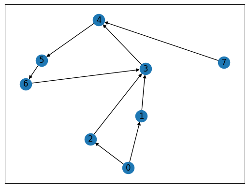
このグラフを描画すると、以下のようになります。

import matplotlib.pyplot as plt

# Compute the layout
pos = nx.spring_layout(inst_G)
nx.draw_networkx(inst_G, pos, with_labels=True)
plt.show()

JijZeptSolverで解く

jijzept_solverを用いて、この問題を解きましょう。

import jijzept_solver

instance = problem.eval(instance_data)
solution = jijzept_solver.solve(instance, solve_limit_sec=1.0)

解の可視化

そして、得られた解を表示してみましょう。

df = solution.decision_variables_df
solution_y = df[df["name"] == "y"]["value"].to_list()
solution_x = df[(df["name"] == "x") & (df["value"] == 1)]["subscripts"].to_list()
# get the set of vertices of y == 1
vertices = [i for i, _ in solution_x]
# set vertices colors
node_colors = ["gold" if i in vertices else "gray" for i in range(inst_num_V)]
# Create a figure with two subplots
fig, (ax1, ax2) = plt.subplots(1, 2, figsize=(10, 5))
# plot the initial graph
nx.draw_networkx(inst_G, pos=pos, with_labels=True, ax=ax1)
ax1.set_title('Initial Graph')
plt.axis('off')
ax1.set_frame_on(False) # Remove the frame from the first subplot
# plot the graph
nx.draw_networkx(inst_G, pos, node_color=node_colors, with_labels=True)
plt.axis('off')
ax2.set_title('Directed Feedback Graph')
plt.show()

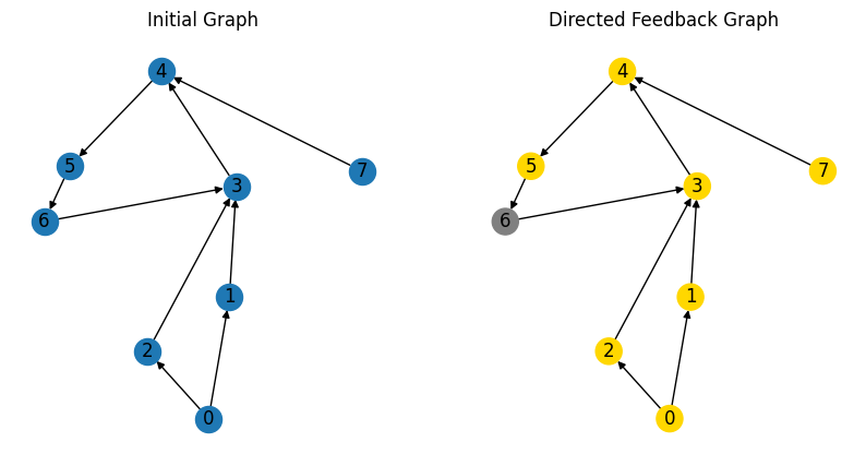
期待通り、JijZeptSolverが最小サイズのフィードバック集合を見つけることができました。
最後に、無向フィードバック頂点集合問題とフィードバック辺集合問題について触れておきましょう。 無向フィードバック頂点集合問題は次のようなものです。 無向グラフにおいて、頂点を取り除いたときに、その結果として出来たグラフが非巡回グラフになるような最小の頂点集合を見つける問題です。 これは最小スパニングツリー問題と非常に良く似ていますが、次数制約や接続制約がありません。 そして先ほどと違う点は、辺を取り除くことができないということです。 フィードバック辺集合問題は、有向グラフが与えられたときに、辺を取り除いて得られるグラフが有向非巡回グラフとなるような最小の辺集合を見つける問題です。 有向フィードバック頂点集合問題と少し似た問題と言えるでしょう。