最小極大マッチング問題

ここではJijZeptSolverとJijModelingを用いて、最小極大マッチング問題を解く方法を紹介します。 この問題は、Lucas, 2014, "Ising formulations of many NP problems" 4.5. Minimal Maximal Matchingでも触れられています。

最小極大マッチング問題とは

最小極大マッチング問題は、グラフにおけるマッチング問題の一つです。 グラフの辺の中で、他のどの辺とも頂点を共有しないような辺集合を探す問題となります。

無向グラフを\(G=(V, E)\)とし、辺の中で色付けされたものを\(C \subseteq E\)のように書くことにしましょう。 \(C\)に対する制約は次のようになります。

1. \(C\)に含まれるどの相異なる2つの辺も、同じ頂点を共有してはならない（マッチング性）

2. \(C\)の辺が結ぶ頂点の集合を\(D\)と書いたとき、\((u, v) \in E\) ならば、\(u, v \in (V \setminus D)\)であってはならない（極大性）

2番目が極大性に相当する理由は、\(u, v \in (V \setminus D)\)である時、\(C\)に辺\((u, v)\)を追加してもマッチング性が保たれるからです。

最小極大マッチングは、この二つの制約を満たすような辺集合\(C\)のうち、最も辺の数が少ないものを求める問題です。

例題

例として、\(V=\{1, 2, 3, 4, 5\}\)と\(E=\{(1, 2), (1, 3), (2, 3), (3, 4), (4, 5)\}\)を持つようなグラフ\(G=(V, E)\)について考えましょう。 極大マッチングを見つけるために、まずはマッチングとして空集合を用意します。 そして、マッチング性を破ることなく辺を追加することができなくなるまで、辺をその集合に追加していきます。

ここで考えているような小さなグラフでは、試行錯誤を繰り返すことで、人の手で最小極大マッチングを見つけることができるかもしれません。 この場合の答えは、\(\{(1, 2), (3, 4)\}\)または\(\{(1, 3), (4, 5)\}, \{(2, 3), (4, 5)\}\)となります。

数理モデル

辺\(e\)を色づけするかどうかを表すバイナリ変数を\(x_e\)を導入します。 これは、\(e\)が色付けされるとき1、そうでないとき0となるような変数です。 また、頂点\(v\)が\(C\)の辺に繋がれているとき1、そうでないとき0となるようなバイナリ変数\(y_v\)も導入します。

制約 1: \(x\)と\(y\)の関係式

\(E_v\)を、頂点\(v\)につながる辺の集合としましょう。

2つのバイナリ変数\(x\)と\(y\)の定義から、\(y_v = 1\)であることと\(\sum_{e \in E_v} x_e \ge 1\)であることは同値です。 いま、1つ目の条件（マッチング性）によって\(\sum_{e \in E_v} x_e \le 1\)が成り立っている必要がありますから、以下のような式を立てることができます。

\[ \quad y_v = \sum_{e \in E_v} x_e \quad \forall v, \]

制約 2: 選ばれなかった全ての辺は、選ばれた辺につながる頂点のうち少なくとも1つにつながれてなければならない

極大性に相当するこの制約を定式化するために、\(1-y_u\)という量を用いましょう。 すると、これは\(u\)が選ばれた辺につながっている場合に0となります。 そして\((1-y_u)(1-y_v)\)を全ての辺\((u, v) \in E\)に対して数え上げれば、制約の破れをチェックすることができます (\((1-y_u)(1-y_v)\)>0ならば、辺\((u, v) \in E\)を制約の破れなく選択することができます。)

\[ \quad \sum_{(u,v)\in E} (1-y_u)(1-y_v) = 0. \]

目的関数: マッチングのサイズを最小化する

ここでのサイズとは、選択された辺の数を意味します。

\[ \quad \min \sum_{e \in E} x_e. \]

JijModelingによる定式化

次に、JijModelingを用いて、上述の数式を実装しましょう。 最初に、数理モデルで用いられている変数を定義します。

import jijmodeling as jm

# define problem
problem = jm.Problem('Minimum Maximal Matching')

# define variables
V = problem.Natural('V')
E = problem.Graph('E', dtype=V)
num_E = problem.NamedExpr('num_E', E.len_at(0))
x = problem.BinaryVar('x', shape=(num_E,))
y = problem.BinaryVar('y', shape=(V,))

制約と目的関数

制約と目的関数を実装しましょう。

problem += problem.Constraint(
    'y_x_relation',
    lambda v: y[v] - jm.sum(jm.filter(lambda e: (E[e][0]==v)|(E[e][1]==v), num_E), lambda e: x[e]) == 0,
    domain=V
)
problem += problem.Constraint(
    'unselected_edge',
    jm.sum(num_E, lambda e: (1-y[E[e][0]])*(1-y[E[e][1]]))==0
)

problem += x.sum()

Jupyter Notebook上で、実装した数式を表示してみましょう。

problem

\[\begin{array}{rl} \text{Problem}\colon &\text{Minimum Maximal Matching}\\\displaystyle \min &\displaystyle \sum _{\vec{\imath }}{{{\left(x\right)}}_{\vec{\imath }}}\\&\\\text{s.t.}&\\&\begin{aligned} \text{unselected\_{}edge}&\quad \displaystyle \sum _{e=0}^{num\_{}E-1}{\left(1-{y}_{{E}_{e,0}}\right)\cdot \left(1-{y}_{{E}_{e,1}}\right)}=0\\\text{y\_{}x\_{}relation}&\quad \displaystyle {y}_{v}-\left(\sum _{\substack{e=0\\{E}_{e,0}=v\lor {E}_{e,1}=v}}^{num\_{}E-1}{{x}_{e}}\right)=0\quad \forall v\;\text{s.t.}\;v\in \left\{0,\ldots ,V-1\right\}\end{aligned} \\&\\\text{where}&\\&\text{Decision Variables:}\\&\qquad \begin{alignedat}{2}x&\in \mathop{\mathrm{Array}}\left[num\_{}E;\left\{0, 1\right\}\right]&\quad &1\text{-dim binary variable}\\y&\in \mathop{\mathrm{Array}}\left[V;\left\{0, 1\right\}\right]&\quad &1\text{-dim binary variable}\\\end{alignedat}\\&\\&\text{Placeholders:}\\&\qquad \begin{alignedat}{2}E&\in \mathop{\mathrm{Array}}\left[(-);V\times V\right]&\quad &1\text{-dimensional array of placeholders with elements in }V\times V\\V&\in \mathbb{N}&\quad &\text{A scalar placeholder in }\mathbb{N}\\\end{alignedat}\\&\\&\text{Named Expressions:}\\&\qquad \begin{alignedat}{2}num\_{}E&=\mathop{\mathtt{len\_{}at}}\left(E,0\right)&\quad &\in \mathbb{N}\\\end{alignedat}\end{array} \]

インスタンスの準備

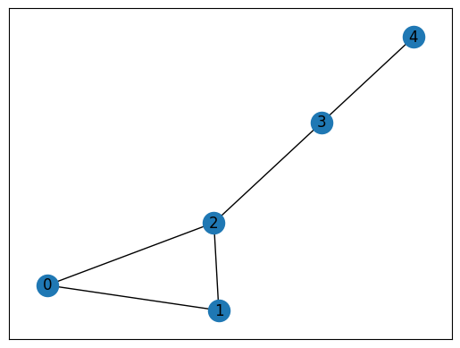
ここでは、先ほど例題として示したグラフを用いましょう。

import networkx as nx

# set empty graph
inst_G = nx.Graph()
V = [0, 1, 2, 3, 4]
# add edges
inst_E = [[0, 1], [0, 2], [1, 2], [2, 3], [3, 4]] 
inst_G.add_edges_from(inst_E)
# get the number of nodes
inst_V = list(inst_G.nodes)
num_V = len(inst_V)
instance_data = {'V': num_V, 'E': inst_E}

このグラフを描画すると、次のようになります。

import matplotlib.pyplot as plt

pos = nx.spring_layout(inst_G)
nx.draw_networkx(inst_G, pos=pos, with_labels=True)
plt.show()

JijZeptSolverで解く

jijzept_solverを用いて、この問題を解きましょう。

import jijzept_solver

instance = problem.eval(instance_data)
solution = jijzept_solver.solve(instance, solve_limit_sec=1.0)

解の可視化

得られた解を可視化してみましょう。

import numpy as np

# get the indices of x == 1
df = solution.decision_variables_df
x_indices = np.ravel(df[(df["name"] == "x") & (df["value"] == 1.0)]["subscripts"].to_list())
# get the indices of y == 1
y_indices = np.ravel(df[(df["name"] == "y") & (df["value"] == 1.0)]["subscripts"].to_list())
# set color list for visualization
cmap = plt.get_cmap("tab10")
# set vertex color
vertex_colors = [cmap(1) if i in y_indices else cmap(0) for i in inst_V]
# set edge color list
edge_colors = ["red" if j in x_indices else "black" for j, _ in enumerate(instance_data["E"])]
# dwaw the figure with two subplots
fig, (ax1, ax2) = plt.subplots(1, 2, figsize=(10, 5))
# plot the initial graph
nx.draw_networkx(inst_G, pos, with_labels=True, ax=ax1)
ax1.set_title('Initial Graph')
plt.axis('off')
ax1.set_frame_on(False) # Remove the frame from the first subplot
# plot the minimum maximal matching graph
nx.draw_networkx(inst_G, pos=pos, node_color=vertex_colors, edge_color=edge_colors, with_labels=True)
plt.axis('off')
ax2.set_title('Minimum Maximal Matching Graph')
# Show the plot
plt.show()

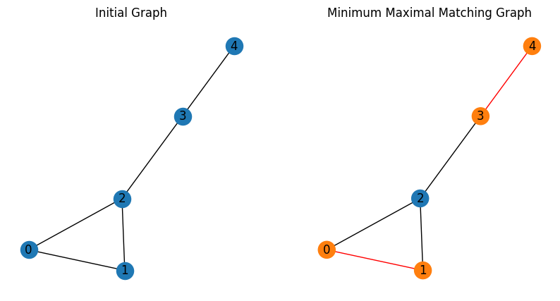
期待通り、最小極大マッチンググラフを得ることができました。