最大次数制約を持つ最小スパニングツリー問題

ここではJijZeptSolverとJijModelingを用いて、最大次数制約を持つ最小スパニングツリー問題を解く方法を説明します。 この問題は、Lucas, 2014, "Ising formulations of many NP problems" 8.1. Minimal Spanning Tree with a Maximal Degree Constraint で触れられています。

最大次数制約を持つ最小スパニングツリー問題とは

最小スパニングツリー問題は、次のように定義されます。 各辺\((uv) \in E\)がそれぞれコスト\(c_{uv}\)を持つような、無向グラフ\(G=(V, E)\)が与えられたとします。 全ての頂点を含むようなツリーである、スパニングツリー \(T \subseteq G\)を構築することを考えます。 もし\(T\)が存在するとき、そのコスト

\[ c(T) = \sum_{(uv) \in E_T} c_{uv} \]

を最小化することを考えるのが、この最小スパニングツリー問題です。 そしてここに、\(T\)に含まれる頂点の次数が\(\Delta\)以下でなければならないという、最大次数制約を加えます。

例題

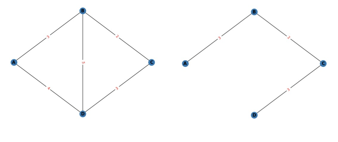
簡単のため、ここでは次のような単純なグラフを見てみましょう。 左グラフにおいて、最大次数が3で制限されるような、最小スパニングツリーを求めてみましょう。 この問題に対する答えは、右のグラフのようになります。 このツリーの重みの総和は8で最小です。 そして最大次数制約も満たされていることがわかります。

数理モデル

辺\(e=(uv)\)が最小スパニングツリー\(T\)に含まれるとき1、そうでないとき0となるようなバイナリ変数\(x_{uv}\)を導入します。

制約 1: 各頂点は最大で\(\Delta\)まで辺を持つことができる

グラフにおけるどの頂点の次数も、\(\Delta\)を超えることはできません。 ツリーでは少なくとも1つの辺を持たなければならないため、各頂点の次数に下界を考える必要があります。

\[ \quad 1 \leq \sum_{(uv),(vu) \in E} x_{uv} \leq \Delta \quad \forall u \in V. \]

\(x_{uv}, x_{vu}\)についての総和であることに注意が必要です。

制約 2: ツリーは全ての頂点を含めなければならない

選択された辺は、全ての頂点を含めるような木を形成しなければなりません。 もし\(T\)の辺の合計が\(|V|-1\)より小さいならば、\(T\)は全ての辺を含めることができません。 そして\(T\)の辺の合計が\(|V|-1\)より大きければ、\(T\)はツリーではなくなります (この場合、グラフにループが存在することになります。)

\[ \quad \sum_{(uv) \in E} x_{uv} = |V|-1. \]

制約 3: 切断制約

この制約により、解のグラフがバラバラでなく接続されており、非巡回グラフとなることを保証します。

\[ \quad \sum_{(uv) \in E(S)} x_{uv} \leq |S| - 1 \quad \forall S \subset G, \]

ここで\(S\)はグラフ\(G\)の部分グラフ、そして\(E(S)\)は\(S\)内に含まれる辺の集合です。

目的関数

\(T\)の重みの総和を最小化する目的関数を設定します。

\[ \quad \min \sum_{uv \in E} c_{uv}x_{uv}. \]

JijModelingによるモデル化

次に、JijModelingを用いて数理モデルを実装しましょう。 最初に、上述の数理モデルに必要な変数を定義します。

import jijmodeling as jm

# define problem
problem = jm.Problem("minimum spanning tree with a maximum degree constraint")

# define variables
V = problem.Natural('V')  # number of vertices
E = problem.Graph('E')  # set of edges
num_E = problem.DependentVar('num_E', E.len_at(0))
C = problem.Float('C', shape=(V, V))  # cost between each vertex
D = problem.Natural('D')  # number of degrees
S = problem.Float('S', ndim=3, jagged=True)  # list of set of subgraph edges
num_S = problem.DependentVar('num_S', S.len_at(0))
S_nodes = problem.Natural('S_nodes', shape=(num_S,))  # list of number of subgraphs vertices

x = problem.BinaryVar('x', shape=(num_E,))

制約と目的関数を実装しましょう。

problem += problem.Constraint(
    'const1-1',
    lambda v: jm.filter(lambda e: (E[e][0]==v)|(E[e][1]==v), num_E).map(lambda e: x[e]).sum() >= 1,
    domain=V
)
problem += problem.Constraint(
    'const1-2',
    lambda v: jm.filter(lambda e: (E[e][0]==v)|(E[e][1]==v), num_E).map(lambda e: x[e]).sum() <= D,
    domain=V
)
problem += problem.Constraint('const2', x.sum() == V-1)
problem += problem.Constraint(
    'const3',
    lambda i_s: jm.sum(S[i_s].len_at(0), lambda e_s: x[e_s]) <= S_nodes[i_s] - 1,
    domain=num_S
)
problem += jm.sum(num_E, lambda e: C[E[e][0], E[e][1]] * x[e])

Jupyter Notebook上で、実装した数理モデルを表示してみましょう。

problem 

\[\begin{split}\begin{array}{rl} \text{Problem}\colon &\text{minimum spanning tree with a maximum degree constraint}\\\displaystyle \min &\displaystyle \sum _{e=0}^{num\_{}E-1}{{C}_{{{E}_{e}}_{0},{{E}_{e}}_{1}}\cdot {x}_{e}}\\&\\\text{s.t.}&\\&\begin{aligned} \text{const1-1}&\quad \displaystyle \sum _{\substack{e=0\\{{E}_{e}}_{0}=v\lor {{E}_{e}}_{1}=v}}^{num\_{}E-1}{{x}_{e}}\geq 1\quad \forall v\;\text{s.t.}\;v\in \left\{0,\ldots ,V-1\right\}\\\text{const1-2}&\quad \displaystyle \sum _{\substack{e=0\\{{E}_{e}}_{0}=v\lor {{E}_{e}}_{1}=v}}^{num\_{}E-1}{{x}_{e}}\leq D\quad \forall v\;\text{s.t.}\;v\in \left\{0,\ldots ,V-1\right\}\\\text{const2}&\quad \displaystyle \sum _{\vec{\imath }}{{{\left(x\right)}}_{\vec{\imath }}}=V-1\\\text{const3}&\quad \displaystyle \sum _{e\_{}s=0}^{\mathop{\mathtt{len\_{}at}}\left({S}_{i\_{}s},0\right)-1}{{x}_{e\_{}s}}\leq {S\_{}nodes}_{i\_{}s}-1\quad \forall i\_{}s\;\text{s.t.}\;i\_{}s\in \left\{0,\ldots ,num\_{}S-1\right\}\end{aligned} \\&\\\text{where}&\\&\text{Decision Variables:}\\&\qquad \begin{alignedat}{2}x&\in \mathop{\mathrm{Array}}\left[num\_{}E;\left\{0, 1\right\}\right]&\quad &1\text{-dim binary variable}\\\end{alignedat}\\&\\&\text{Placeholders:}\\&\qquad \begin{alignedat}{2}C&\in \mathop{\mathrm{Array}}\left[V\times V;\mathbb{R}\right]&\quad &2\text{-dimensional array of placeholders with elements in }\mathbb{R}\\D&\in \mathbb{N}&\quad &\text{A scalar placeholder in }\mathbb{N}\\E&\in \mathop{\mathrm{Array}}\left[(-);\mathbb{N}\times \mathbb{N}\right]&\quad &1\text{-dimensional array of placeholders with elements in }\mathbb{N}\times \mathbb{N}\\S&\in \mathop{\mathrm{JaggedArray}}\left[(-)\times (-)\times (-);\mathbb{R}\right]&\quad &3\text{-dimensional array of placeholders with elements in }\mathbb{R}\\S\_{}nodes&\in \mathop{\mathrm{Array}}\left[num\_{}S;\mathbb{N}\right]&\quad &1\text{-dimensional array of placeholders with elements in }\mathbb{N}\\V&\in \mathbb{N}&\quad &\text{A scalar placeholder in }\mathbb{N}\\\end{alignedat}\\&\\&\text{Dependent Variables:}\\&\qquad \begin{alignedat}{2}num\_{}E&=\mathop{\mathtt{len\_{}at}}\left(E,0\right)&\quad &\in \mathbb{N}\\num\_{}S&=\mathop{\mathtt{len\_{}at}}\left(S,0\right)&\quad &\in \mathbb{N}\\\end{alignedat}\end{array} \end{split}\]

インスタンスの準備

NetworkXを用いて、グラフを準備しましょう。 例として、ランダムな完全グラフ (全ての頂点がお互いに接続されているようなグラフ) を作成しましょう。

import itertools
import networkx as nx
import numpy as np

np.random.seed(seed=0)

# set the number of vertices
inst_V = 5
# set the number of degree
inst_D = 2

# set the probability of rewiring edges
p_rewire = 0.2
# set the number of nearest neighbors
k_neighbors = 4
# create a connected graph
inst_G = nx.connected_watts_strogatz_graph(inst_V, k_neighbors, p_rewire)
# add random costs to the edges
for u, v in inst_G.edges():
    inst_G[u][v]['weight'] = np.random.randint(1, 10)

# create a 2D array for the costs
inst_C = np.zeros((inst_V, inst_V))
for u, v in inst_G.edges():
    inst_C[u][v] = inst_G[u][v]['weight']
    inst_C[v][u] = inst_G[u][v]['weight']
# set diagonal elements to infinity
np.fill_diagonal(inst_C, np.inf)

# get information of edges
inst_E = [list(edge) for edge in inst_G.edges]

# get subgraphs and their edges
sub_nodes = []
sub_edges = []
# get connected subgraphs that have at least 2 nodes and have less nodes than the original graph
for num_nodes in range(2, inst_G.number_of_nodes()):
    for comb in (inst_G.subgraph(selected_nodes) for selected_nodes in itertools.combinations(inst_G, num_nodes)):
        if nx.is_connected(comb):
            sub_edges.append(comb.edges)
            sub_nodes.append(comb.nodes)
inst_S = [list(edgeview) for edgeview in sub_edges]
inst_S = [[list(t) for t in inner_list] for inner_list in inst_S]  # convert tuples into lists
# get the number of vertices in each subgraph
inst_S_nodes = [len(x) for x in sub_nodes]

instance_data = {'V': inst_V, 'D': inst_D, 'E': inst_E, 'C': inst_C, 'S': inst_S, 'S_nodes': inst_S_nodes}

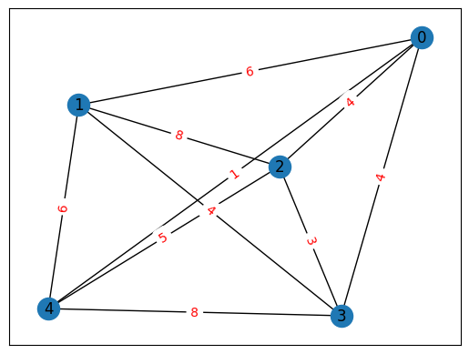
ここで作られたグラフを表示してみます。

import matplotlib.pyplot as plt

pos = nx.spring_layout(inst_G)
nx.draw_networkx(inst_G, pos, with_labels=True)
edge_labels = nx.get_edge_attributes(inst_G, 'weight')
nx.draw_networkx_edge_labels(inst_G, pos, edge_labels=edge_labels, font_color='red')

plt.show()

Solve by JijZeptSolver

この問題をjijzept_solverを用いて解きましょう。

import jijzept_solver

instance = problem.eval(instance_data)
solution = jijzept_solver.solve(instance, solve_limit_sec=1.0)

解の可視化

得られた解を可視化してみましょう。

# get the indices of x == 1
df = solution.decision_variables_df
x_indices = df[df["value"]==1]["subscripts"].to_list()# set edge color list (x==1: black, x==0: white)
inst_E = np.array(inst_E)
mask = inst_E[:, 0] > inst_E[:, 1]
inst_E[mask] = inst_E[mask][: , : :-1]
edge_colors = np.where(np.isin(np.arange(len(inst_E)), x_indices), 'black', 'white').tolist()
# draw figure
plt.subplot(121)
plt.axis('off')
nx.draw(inst_G, pos, with_labels=True, font_weight='bold')
nx.draw_networkx_edge_labels(inst_G, pos, edge_labels=edge_labels, font_color='red')
plt.subplot(122)
plt.axis('off')
inst_H = inst_G.copy()
for i in range(len(inst_H.edges)):
    if edge_colors[i] == 'white':
        inst_H.remove_edge(*list(inst_G.edges)[i])
nx.draw(inst_H, pos, with_labels=True, font_weight='bold')
nx.draw_networkx_edge_labels(inst_H, pos, edge_labels=nx.get_edge_attributes(inst_H, 'weight'), font_color='red')

{(0, 4): Text(0.004709307600212931, 0.0906234383694593, '1'),
 (0, 2): Text(0.49403114046146035, 0.5678539174374728, '4'),
 (1, 3): Text(-0.10110844399733399, -0.15848411239151816, '4'),
 (2, 3): Text(0.3237174278353945, -0.36524810117169304, '3')}

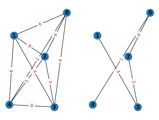
期待通り、最大次数制約を満たす最小スパニングツリーを得ることができました。
ここで紹介した問題の高度な発展として、シュタイナーツリー問題というものがあります。 この問題は次のようなものです。 辺のコスト\(c_{uv}\)が与えられたとき、頂点の部分集合\(U \subset V\)に対して最小スパニングツリーを考えます。 ここで\(U\)に含まれないノードの使い方は、自由とします。 この問題を解くには、最小スパニングツリー問題と同じハミルトニアンを用いることができますが、頂点\(v\)が\(U\)に含まれるかどうかを表す追加のバイナリ変数\(y_v\)を用いる必要があります。